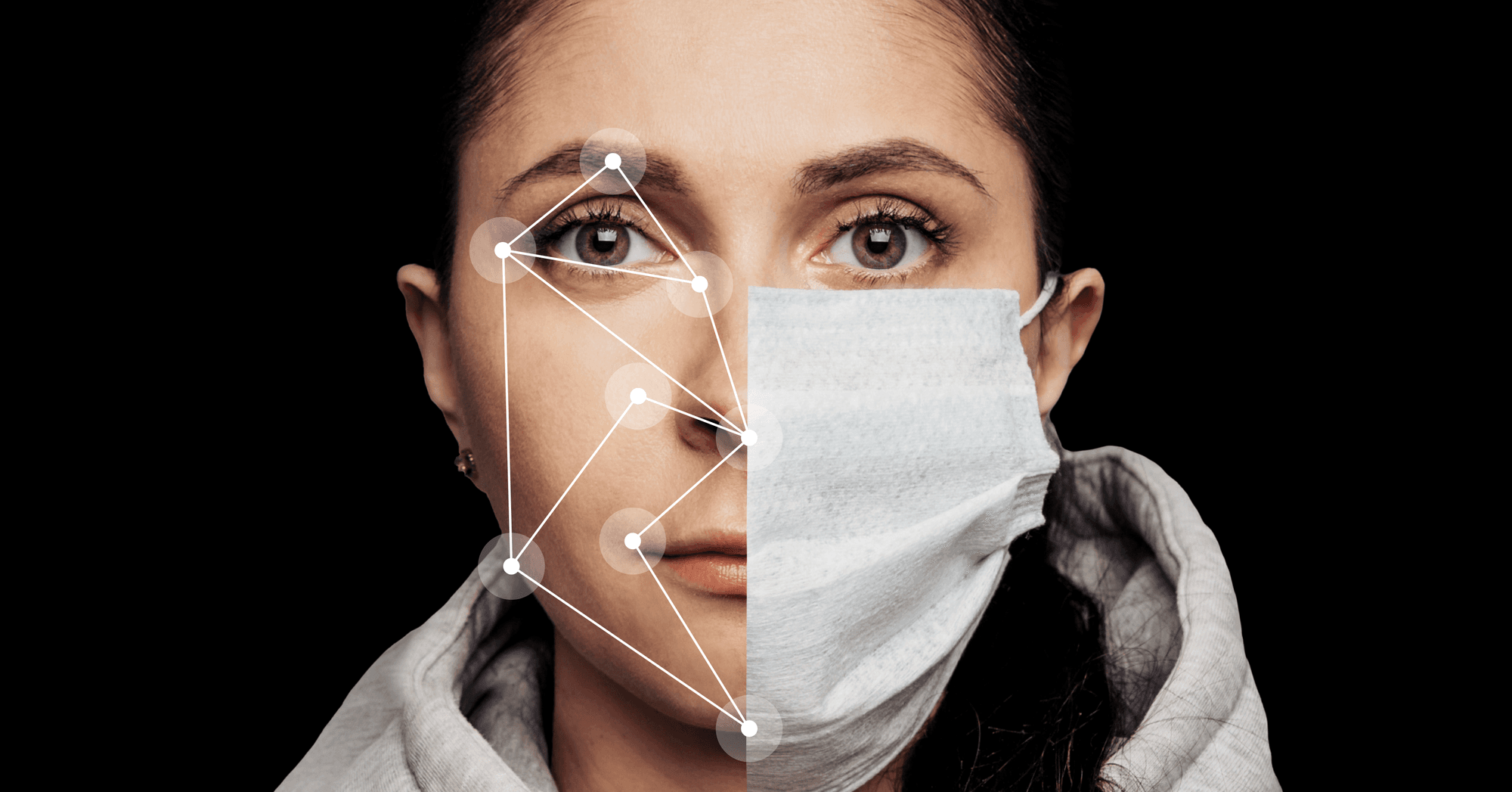
Want to know how we crafted an ML tool that virtually removes the mask from a person’s face?
This article will guide you through the whole process of crafting the deep learning ML model — from the initial setup, data gathering and proper model selection to the training and fine-tuning.
Before we dive in, let’s define the nature of our task. The problem we are trying to solve can be viewed as image inpainting, which is generally considered to be the process of restoring damaged images or filling in the missing parts. You can see examples of image inpainting below; the input images had white gaps which were restored.
Examples of image inpainting using Partial Convolutions. [Source]
With that settled, one more note before we start: Apart from this article, we’ve also prepared a GitHub account with everything you need already implemented, as well as the Jupyter Notebook `mask2face.ipynb` — where you can run everything mentioned here in just a few simple clicks, training your own neural network!
Let’s begin.
Preconditions
First of all, if you’d like to follow all of the steps described in this article on your computer, you can clone this project from our GitHub.
Let’s start with preparing the virtual environment for our Python project. You can of course use any virtual environment you like, just make sure to install all necessary dependencies from environment.yml and requirements.txt. If you are not familiar with virtual environments or Conda, check out this nice article for some info. And if you are familiar with Conda, you can go ahead and initialize the Conda environment by running the following commands from the directory where you cloned the GitHub project:
conda env create -f environment.yml
conda activate mask2face
Now that you have an environment with all necessary dependencies, let’s define our goals and objectives. For this particular project, we want to create an ML model that can show us what a person wearing a face mask looks like without that mask. Our ML model has one input — an image of a person with a face mask on; and one output — an image of a person without the mask.
Implementation
High-level ML Pipeline
The whole project is nicely represented as a high-level pipeline in the following image.
We start with a dataset of faces with precomputed face landmarks that are processed through the mask generator. It uses the landmarks to position the mask on the face. Now that we have the dataset with pairs of images (with and without the mask), we can continue with defining the architecture of the ML model. Finally, the last part of the pipeline is to find the best loss function and all necessary scripts to put everything together, so we can train and evaluate the model.
Data Generation
To train the deep learning model, we need a lot of data. In this case, we need a lot of pairs of input and output images. It is of course not practical to gather both input and output images of the same person with and without a mask. We can do better and act much faster.
There are many datasets of human face images used mainly for the training of face detection algorithms. We can take a dataset like this, paint a mask onto the faces and voilà — we have our image pairs.
We experimented with two different datasets. One database we used is Labeled Faces in the Wild from the University of Massachusetts [1]. Here is the 104MB gzipped tar file with the whole dataset of over 5,000 images. This dataset suits our case well, since it contains images with a focus on human faces. However, for the final results, we used the CelebA dataset, which is larger (200,000 samples) and contains higher quality images.
Next, we need to locate facial landmarks so we can place the mask in the right place. To do so, we used a pretrained dlib facial landmark detector. You can use any other similar dataset, just make sure that you can find the precomputed face landmark points (this GitHub repo can be a good source) or compute landmarks by yourself.
Mask Generator
Initially, we started with a simple implementation of a mask generator by placing a polygon on the face with a randomized distance of the polygon vertices from the face landmarks. This way, we could quickly generate a simple dataset and test if the idea behind this project is valid. Once established that it really is valid, we looked for a more robust solution that would better capture real-world scenarios.
There is a great GitHub project, Mask The Face, that already solves the mask generation problem. It estimates mask position from face landmark points, estimates face tilt angle to select the best fitting mask from the database and, finally, places the mask on the face. The database of available masks includes surgical masks, cloth masks with a variety of colors and textures, several types of respirators and even gas masks.
import matplotlib.pyplot as plt
import matplotlib.image as mpimg
from utils.data_generator import DataGenerator
from utils.configuration import Configuration

# You can update configuration.json to change behavior of the generator
configuration = Configuration()
dg = DataGenerator(configuration)

# Generate images
dg.generate_images()

# Plot a few examples of image pairs
n_examples = 5
inputs, outputs = dg.get_dataset_examples(n_examples)
f, axarr = plt.subplots(2, n_examples, figsize=(20,10))
for i in range(len(inputs)):
    axarr[1, i].imshow(mpimg.imread(inputs[i]))
    axarr[0, i].imshow(mpimg.imread(outputs[i]))
Architecture
Now that we have a dataset prepared, it is time to work on a deep neural network model architecture. This is definitely a situation where no one can claim there’s an objectively “best” option.
Selecting the proper architecture always depends on many factors, like time requirements (do you want to process videos in real-time or do you want to pre-process a batch of images offline?), hardware requirements (should the model run on a cluster of high-power GPUs or will it run on a low-power mobile device?) and many more. It is always about finding the right parameters and setting for your specific case.
If you want to get a bit philosophical about this issue, you can read more in this KDnuggets post or in this scholarly article.
Convolutional Neural Network
A Convolution Neural Network (CNN) is a type of neural network architecture that utilizes convolution kernel filters. They are suitable for a wide range of problems — like time series analysis, natural language processing and recommendation systems — but are primarily used in anything image-related, like object classification, image segmentation, image analysis and image inpainting.
The core of a CNN is the convolution layer that is capable of detecting visual features of the input images. When we stack multiple convolution layers on top of each other, they have a tendency to detect different features. The first layers usually extract more complex features, such as corners or edges. As you move deeper into the CNN, the layers start detecting higher-level features, such as objects, faces and more.
For a more detailed description of CNNs, see this TechTalks article or these Stanford notes.
Example of CNN architecture. [Source]
The image above shows an example of a CNN for image detection. This is not the exact problem we are trying to solve, but the CNN architecture is a necessary building block for any inpainting architecture.
ResNet Blocks
Before we get to some inpainting architectures, let’s discuss the final helpful building blocks. They are called ResNet blocks, or residual blocks. In traditional neural networks or CNNs, each layer is connected to the next layer. In a network with residual blocks, layers are connected to the next layers as well, but also to two or more layers away. We introduced the ResNet blocks to further improve the performance, as will be described later.
ResNet building block. Source [7]
Neural Networks are capable of approximating any function and we could think that increasing the number of layers will increase the accuracy of the approximation. However, thanks to problems like vanishing gradient or the curse of dimensionality, adding more layers will, at some point, stop increasing the performance and can actually start decreasing it. That is why a lot of research has been dedicated to these problems — and one of the best performing solutions is the residual block.
Residual blocks allow the flow of information from the initial layers to the next layers using the skip connections or the identity function. By giving the Neural Network the ability to use the identity function, we can build networks with better performance than by just adding more layers. You can read more about ResNet and its variants here: [8]
Encoder-Decoder
The Encoder-Decoder architecture consists of two separate neural networks: The Encoder extracts a fixed-length representation of the input (embedding), and the Decoder generates output from this representation.
Encoder-Decoder network for image segmentation. Source [6]
You can notice that the encoder part looks very similar to the CNN described in the previous section. Proven classification CNNs are often used as the base of the Encoder or even directly as the Encoder, without the last (classification) layer. This architecture is capable of generating new images, which is exactly what we need. The performance, however, is not that great — so let’s look at something better.
U-net
U-net is convolutional neural network architecture developed originally for image segmentation [2], but it eventually became useful for many more tasks, such as image inpainting or image colorization.
U-net architecture from the original article. Source [2]
Our previous mention of the ResNet block had an important reason. The fact is, combining ResNet blocks with the U-net architecture arguably had the biggest impact on the overall performance. You can see the architecture of the added ResNet blocks in the image below.
Upscale ResNet block (top) and downscale ResNet block (bottom) used in the U-net.
When you compare the U-net architecture above with the Encoder-Decoder architecture from the previous section, they look very similar — but there’s one critical difference. U-net implements something called ‘skip connections’, which propagates identity from deconvolution blocks to corresponding upsampling blocks on the other side (gray arrows on the image above). This is an improvement from Encoder-Decoder in two notable ways.
First, the skip connections are known to speed up the learning process and help tackle the vanishing gradient problem [5]. Second, they pass the information from the encoder directly to the decoder, helping recover information loss during downsampling. We can say that they can propagate all parts of the image outside of the face mask that we want to keep unchanged, while also helping with the generation of the part of the face beneath the mask.
This is exactly what we need! Skipping connections will help preserve the parts of the input that we want to propagate to the output, while the Encoder-Decoder part of the U-net will detect the mask and replace it with the mouth underneath.
Loss Functions
The choice of the loss function is one of the most important problems you need to solve. Working with the correct loss function can mean the difference between a great performing model and a barely functioning one. That is why we spend a lot of time choosing the best option. Let’s discuss several possibilities.
Mean Square Error (MSE) and Mean Absolute Error (MAE)
Both MSE and MAE are loss functions based on the per-pixel difference between the image generated by our model and the ground truth image from the dataset before applying the mask onto the face. This seems like exactly what we need, but we are not trying to train the model that can pixel-perfectly recreate what is hidden under the mask.
We want our model to understand that beneath a mask are a mouth and a nose, and even to possibly understand the emotion from what is not hidden (for example, the eyes) to generate a sad 😔, happy 😃 or perhaps surprised face 😲. This means that even output that does not capture every pixel perfectly can, in fact, be a great result; and, more importantly, it can learn how to generalize on any face, not just the ones in the training dataset. That is why we get much better results using different loss functions.
Structural Similarity Index (SSIM)
SSIM is a metric used for measuring the similarity between two images. Proposed by Wang et al. (2004) [3], it focuses on solving the exact problems we have with MSE/MAE. It gives us a numeric value expression of just how much two images resemble each other, instead of how many pixels have the same intensity. It does so by comparing three measurements between images: luminance, contrast and structure. The final score is the weighted combination of all three measurements from 0 to 1, where 1 means completely similar images.
The following images illustrate the problem with MSE. The top left image is the original image without any modifications. All other images are distorted in a different way. The Mean Square Error between the original image and every other image is always roughly the same (around 480), while the SSIM varies a lot. For example, the blurred image and the segmented image are definitely less similar to the original image than any other, but the MSE is almost the same — despite the loss of facial features and details on the head and dress. On the other hand, the color-shifted image and the image with contrast stretch are very similar to the original image in human eyes (and SSID metric), but the MSE disagrees.
Results
Training
We trained our model with U-net architecture using the ADAM optimizer and SSIM loss function. We split the dataset into a testing part (1,000 images), training part (80% of the rest of the dataset) and validation part (80% of the rest of the dataset). Our first experiments produced decent but not very sharp output images for several testing images. It was time to experiment with architecture and loss functions to boost the performance. Here are some of the changes we tried:
Number of Layers and Sizes of Convolution Filters
More convolution filters and a deeper network mean much more parameters (while 2D convolution layer with size [8, 8, 256] have 0.59 million parameters, layer with size [4, 4, 512] have 2.3 million parameters ) and more training time. Since the depth and number of filters in each layer is the input parameter for the constructor of our model’s architecture, it is super easy to experiment with different values.
After some time, we found that, for us, the best balance between performance and model size is the following setup:
# Train model with different number of layers and filter sizes
from utils.architectures import UNet
from utils.model import Mask2FaceModel

# Feel free to experiment with the number of filters and their sizes
filters = (64, 128, 128, 256, 256, 512)
kernels = ( 7,   7,   7,   3,   3,   3)
input_image_size=(256, 256, 3)
architecture = UNet.RESNET
training_epochs = 20
batch_size = 12

model = Mask2FaceModel.build_model(architecture=architecture, input_size=input_image_size, filters=filters, kernels=kernels)
model.summary()
model.train(epochs=training_epochs, batch_size=batch_size, loss_function='ssim_l1_loss')
We did some experimenting, and the setup in the code block above worked the best for us.
Now that we have trained and tuned the model with all the tweaks mentioned above, let’s look at some results!
Left: Input for our model, Middle: Input images without the mask (expected output), Right: Output of our model
As you can see, the proposed network produces great results on our testing data. The network is capable of generalizing, and it also appears that it can spot emotions well enough to generate smiling or sad faces. On the other hand, there is certainly some room for improvement.
Ideas for Additional Improvements
Even though the results of our U-net with ResNet block are great, we can see that the generated image under the mask is not very sharp. One way to fix that is to extend our network with a refinement network, as described in [4] and shown in the following image. There are, however, a few other improvements that can be done.
Improving Dataset
As we experienced during the experiments, the choice of the dataset can have a significant impact on results. As a next step, we would combine different datasets to have more variability of samples, mimicking real-world data even better. Another thing that could be improved is the way masks are combined with faces, making them look more natural. A good source of inspiration could be [12].
Variational Autoencoder
We already mentioned the Encoder-Decoder architecture, where the encoder part maps the input image into embedding. We can view the embedding as a single point in a multidimensional latent space. The Variational Autoencoder is, in many ways, similar to the Encoder-Decoder; the main difference is probably that, with the Variational Autoencoder, mapping is done into multivariate normal distribution around a point in the latent space. This means that the encoding is, by design, continuous and allows for much better random sampling and interpolation. This could help a lot with significantly smoother images generated on the output of the network.
Generative Adversarial Networks
GANs are capable of generating results indistinguishable from real photographs. That is mainly thanks to a completely different approach to learning. While our current model is trying to minimize loss during the training, GANs are composed of two separate neural networks: generator and discriminator. The generator generates output images, while the discriminator tries to decide whether the image is real or generated by the generator.
During the learning, both networks are dynamically updated to perform better and better until, in the end, the discriminator is incapable of deciding whether the generated image is real or not, and the generator is producing images indistinguishable from real ones.
Example of GANs creating mixed face from Source A and B. [9]
The GANs results are great, but they usually have problems with convergence during training and it takes a long time to train them. GAN models are also usually much more complex due to a large number of parameters, and they are not very suitable for export to mobile phones.
Concat ImageNet and FaceNet Embedding
In many ways, U-net’s bottleneck layer serves as a feature extraction embedding. Articles like [10], [11] suggest that concatenating embeddings of different networks can improve overall performance.
We tried to combine our embedding (the bottleneck layer) with two different embeddings from ImageNet and FaceNet. Our expectation was that this could add more information about the human face and its features to help the upsampling part of the U-net with face restoration. This definitely improved performance but, on the other hand, it made the whole model much more complex, and the performance boost was much smaller than using the other improvements mentioned in the Training section.
Conclusion
Face reconstruction of this sort comes with many challenges. As we uncovered, getting the best results required a creative approach of combining various datasets and techniques. Many specifics such as occlusion, illumination and pose invariance must be properly addressed. Failing to do so causes a notable decline in accuracy — in both traditional handcrafted solutions and deep neural networks, as the solution may end up working with a single distribution of photos.
But those challenges were exactly why we found this project appealing.
The reason we set out to create Mask2Face is a prime example of our Data Science department. We observe what’s going on in the world (mask detection) and look for the less-frequented path (taking the mask off). The more difficult the task, the greater the learning experience. A foundational role of data science is to tackle the seemingly impossible, and we always want to do that mindset justice.
It is our pleasure to leverage STRV’s Computer Vision and other expertise on our client projects. If you’re considering our help, you may be interested in our other past work — like the custom AI solution we built for Cinnamon in just four months. And if you’re a fellow engineer, please feel free to reach out to us with any questions, or to share the results of your own work. We’re always happy to start up a discussion.
Bonus: Export to Mobile Phones
We defined the architecture with the possible use of mobile phones on our minds. That is why we used architecture that can produce great results even with a smaller number of parameters (that mobile phones can handle). We may revisit this topic in another article but, if you are interested now, we recommend reading our Training Your Object Recognition Model from Scratch article.
Sources
[1] http://vis-www.cs.umass.edu/lfw/
[2] https://arxiv.org/abs/1505.04597
[3] Wang, Zhou; Bovik, A.C.; Sheikh, H.R.; Simoncelli, E.P. (2004-04-01). "Image quality assessment: from error visibility to structural similarity". IEEE Transactions on Image Processing
[4] Elharrouss, O., Almaadeed, N., Al-Maadeed, S. et al. “Image Inpainting: A Review”. Neural Process Lett 51, 2007–2028 (2020). https://doi.org/10.1007/s11063-019-10163-0
[5] Adaloglou, Nikolas. "Intuitive Explanation of Skip Connections in Deep Learning". (2020) https://theaisummer.com/skip-connections/
[6] Hyeonwoo Noh, Seunghoon Hong and Bohyung Han. “Learning Deconvolution Network for Semantic Segmentation”. (2015) https://arxiv.org/abs/1505.04366
[7]. K. He, X. Zhang, S. Ren, and J. Sun. Deep residual learning for image recognition. arXiv preprint arXiv:1512.03385,2015.
[8] https://towardsdatascience.com/an-overview-of-resnet-and-its-variants-5281e2f56035
[9] T. Karras, S. Laine and T. Aila. A Style-Based Generator Architecture for Generative Adversarial Networks. arXiv preprint arXiv:1812.04948,2019
[10] Danny Francis, Phuong Anh Nguyen, Benoit Huet and Chong-Wah Ngo. Fusion of Multimodal Embeddings for Ad-Hoc Video Search. ICCV 2019
[11] Xin Ma, Xiaoqiang Zhou, Huaibo Huang, Zhenhua Chai, Xiaolin Wei and Ran He. Free-Form Image Inpainting via Contrastive Attention Network. arXiv preprint arXiv:2010.15643, 2020
[12] https://medium.com/neuromation-blog/neuronuggets-cut-and-paste-in-deep-learning-a296d3e7e876

